Study Design
‘How many probes should I place in how many sections?’ is a frequent question that ‘stereologists’ are confronted with – and one that they often are less qualified answering than the person asking.
There are several recommended schools of thought into how much work should be done to achieve a desired level of accuracy. These approaches are discussed below. They each have their own merits.
The oversampling-subsampling approach
Few investigators would be comfortable with a the idea of using a sampling scheme in which the selected sections frequently miss important anatomical features of the structure of interest, and in which probes rarely ‘hit’ the objects whose properties are to be estimated. Sampling schemes which are free of these faults are good “starting schemes” and will often, when formally assessed using CE estimators, typically return methodological contributions to variance which are ‘good enough’ and often ‘better than necessary’. The choice of sampling parameters often depends on a sufficient knowledge of the structure of interest, which can not be substituted for by stereological theory.
This “starting scheme” is at least a good beginning for a more rational study design. If it is judged that, e.g., every n th section would seem appropriate and that probes should be placed at m um x, y-intervals, one may decide to sample two or three animals with, e.g., every ¼ n thsection and with ½ m um intervals. From this larger sample, subsamples can be drawn corresponding to 2, 1, 0.8, 0.66, 0.57, 0.5 … times the originally intended sampling density in terms of sections or probe placement or combinations thereof. The subsample estimates allow us to evaluate:
- How much the estimates actually fluctuate with changes of the sampling intervals, i.e., we obtain a statistical sample of the ‘true’ CE;
- The size and variability of the calculated CEs for a range of sampling intervals, and;
- Which sampling scheme is returning a precision suitable for the purpose of the study.
- Which of the CE estimators and associated factors (see xxx) best predict the observed variability of the subsample estimates and can be used in the assessment of estimate precision in the actual project.
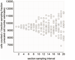
Figure 1 demonstrates the effect of the sampling scheme on the variability of estimates of the total number of cells using the Optical Fractionator. In this example, an increase of the section-sampling interval causes an increase in the variability of the cell population estimates. Here every second section from 2 to 20 is used and estimates are repeated. For instance, a section-sampling interval of 10 means that every tenth section was selected, yielding 10 different estimates of the total numbers of pyramidal cells (with the first estimate based on the analysis of the sections no. 1, 11, 21, …, the second estimate based on the analysis of the sections no. 2, 12, 22, …, and so on). As can be seen, the variation of the estimated total numbers of pyramidal cells increased when increasing the section sampling interval. This variability, originating from estimates made within an individual, adds to the natural variability observed between individuals (from Slomianka and West, 2005).
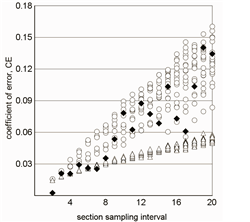
Figure 2.
Figure 2 demonstrates that calculated CEs can vary significantly for a given sampling scheme. In extreme cases, such as the sampling of every 17th section in this investigation of hippocampal neurons, the Gundersen CE varies by almost a factor 3 (open circles show smoothing class m=0, triangles show smoothing class m=1). CE estimates using m=1 are far less variable, but, in this case, they are poor CE estimates for section sampling intervals higher than 8. Comparing the variability of estimates from an oversampling-subsampling approach to CE estimates will show which smoothness factor best approaches the observed variability. For a fixed spacing of probes within the sections, the sampling of every 12th section would be unlikely to produce a CE above 10%. For this section sampling interval, CE estimates using m=0 are better estimators of the ‘true’ CE than CE estimates based on m=1. If a CE of less than 5% was required, at least every 8th section should be sampled. For this and lower section sampling intervals, CEs calculated based on m=1 are better predictors of the methodological contribution to variance than those calculated based on m=0.
The oversampling approach
Many researchers have decided to rely on a reasonable degree of oversampling (which is easy and fast when using automated stereology systems). For instance, numbers of counted cells have been increased to a range of 500 to 1,000 per individual. In this manner, for homogeneously distributed cells, counting approximately 900 cells results in a CE of 0.033. The amount of time necessary to carry out these estimates is typically one day per region of interest, which is a reasonable compromise between the amount of time dedicated to the analysis and the precision of the obtained estimates. Likewise researchers have turned to analyzing volumes using the Cavalieri estimator on the investigation of at least 8 sections and at least 250 counted points. Estimates of mean perikaryal or nuclear volumes on the investigation of a total of at least 500 cells (which typically requires no more than an hour when carried out simultaneously with estimates of total numbers of cells), and estimates of the average length of tubular objects on the investigation of at least 500 intersections of these objects with Space Balls (which typically requires about one day per region of interest).
Finally, oversampling is only one possible empirical solution to the problem of ensuring sufficient precision in an estimate (or group of estimates). For instance, the optimum sampling intensity in a study dealing with total numbers of cells depends not only on the spatial distribution of the cells within the tissue, but also on the kind of statistical analyses to be performed (i.e., comparison of group means, regression analysis, calculation of individual ratios of cell numbers, etc.). Because a general analytical solution to this problem does not exist, we recommend that someone knowledgeable in the field is involved in designing your individual sampling scheme before you start your study. You should then verify your sampling scheme with a pilot study in which you perform oversampling so you can systematically examine the sampling parameters that will yield the most efficient and precise estimation in your design-based stereological study. Your final sampling scheme should address the number of animals or organs to be investigated (an issue not covered in this site), the number of sections to be analyzed, the sampling frequency on the sections to be examined, etc.
For more advice about thinking about precision, please see ‘guide-for-deciding-on-the-precision-of-sampling‘.
REFERENCES:
____________________________________________________________________

Sponsored by MBF Bioscience
developers of Stereo Investigator, the world’s most cited stereology system

