The Gundersen CE is also known as the Matheron transitive technique. This method was originally developed by Matheron at the Ecole Nationale Suiperiere des Mines de Paris. Gundersen and Jensen have extended this work in several papers.
Figure 1. The Gundersen CE formula, also known as the Matheron Transitive Technique.
While this formula looks rather complicated and unlike anything that has to do with the sampling process that was undertaken , what is significant about it is that this method has important predictions about stereological protocols. The most important of these is that the use of systematic uniform random sampling can be efficient and is always no worse than independent random sampling.
The Matheron transitive technique makes an important observation; the samples used in a typical stereological procedure are not independent. This is a mathematical way of saying that sections used were and in a systematically random sampling method.
A typical stereological procedure uses systematically random sampling. This means that instead of choosing every section at random, without regard to what has already been chosen, samples are chosen by choosing the starting one at random and then all other samples are chosen by taking every nth sample after that. For example, suppose that the researcher chooses every 7thsection. This means that the researcher is planning to use 1/7 of the available material. A random number from 1 to 7 is selected. Suppose the random number is 4, then the 4th, 11th, 18th, 25th… sections are used. More on this concept is described in the section on the fractionator.
When using the sampling scheme of every 7th section, the only way the 25th piece can be used is if the starting piece was the 4th. If the 4th piece was used then the 25th must be used. There is clearly a dependency here. The mathematics must take this into account.
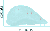
When sampling results are plotted, the plot shows a series of plot points that are plotted at regular intervals just as the material was selected at regular intervals. Sampling introduces random error. This is not a bias, but a fluctuation that is introduced because only a portion of the population is used. There are two issues that are considered by this method. One issue is the variance due to noise. This was formerly called the nugget effect. This is the variance found when sampling within a section. For example, in figure 2 the bars superimposed on the plot show what numbers might be counted on any given section. The variance in the counts on a section occur when the grid with the counting frame are randomly placed on the slices. More on this variance within a section can be found in the section on sampling simulations.
Figure 2. Counts vs. Section Variance.
There is another variance as well. That is the difference between sections. Typically, all sections are different. The difference between sections has a variance that is evident even if exhaustive counting is used on each section. Exhaustive counting reduces each of the vertical bars to a single point. Still there is a difference between the vertical positions of the points in the plot.
The mathematical derivation of the Matheron formula supposes that the dots in the plot can be connected to form a connected curve. Many different curves can be drawn depending on the nature of the curves. These curves fill in the information between the dots. What lies between the dots are the counts from slices that were not used.
It is possible to describe the nature of the curves that can be used to connect the dots. The mathematical nature is described by classes of curves. Two useful classes are considered. These are the m = 0 and the m = 1 classes, also known as the smoothing class. Suffice it say that many conditions the m=1 class is the proper assumption. There are cases in which m = 0 is the correct class. The reason that m = 1 is usually used in biological work is that the m = 1 class is the smooth class without any abrupt jumps in the shape. There are cases in which shapes do have an abrupt change in shape.
A step in the derivation for the formula replaces the curve with piecewise parabolic sections. This important step adds the requirement that there must be at least 3 sections. If only 1 section is used or even if 2 sections are used, it does not matter, the formula cannot be properly used. At least 3 points are required to define a parabola. Studies show that 5 to 15 sections should be used. A possibly useful rule of thumb, really a starting point for a pilot study, is to use 10 to 15 sections for an optical fractionator. Please see If this recommendation is followed, then there is no problem here with the requirement that at least 3 sections are used. Please see ‘CE and Study Design‘ for further discussion of how many sections to use.
REFERENCES
- Gundersen HJ, Jensen EB., J Microsc 1987;147:229.
- Gundersen HJ, Jensen EB, Kieu K, Nielsen J., J Microsc 1999;193:199.
- Mattfeldt, T. J Microsc 1989; 153:301.
____________________________________________________________________

Sponsored by MBF Bioscience
developers of Stereo Investigator, the world’s most cited stereology system

